In this post we will look at steps involved in profiling of the serial code using Intel Vtune Profiler GUI.
Let’s take a simple code which performs some array operations.
#include<stdio.h>
#include<stdlib.h>

#define ARRSIZE 99999999

void print_data(int *C)
{
	int i;
	//print the data
	printf("\tC Array values : ");
	for(i=0;i<ARRSIZE;i++)
	{
		printf("\t%d\n", C[i]);
	}
}

void initialize(int *A, int *B, int *C)
{
	int i;
	//Initialize data to some value
	for(i=0;i<ARRSIZE;i++)
	{
		A[i] = 2*(i+1);
		B[i] = i+1;
	}
	//print_data(C);
}

void add_arrays(int *A, int *B, int *C)
{
	int i;
	for(i=0;i<ARRSIZE;i++)
	{
		C[i] = A[i] + B[i];
	}
	//print_data(C);
}

void sub_arrays(int *A, int *B, int *C)
{
	int i;
	for(i=0;i<ARRSIZE;i++)
	{
		C[i] = A[i] - B[i];
	}
	//print_data(C);
}

void mul_arrays(int *A, int *B, int *C)
{
	int i;
	for(i=0;i<ARRSIZE;i++)
	{
		C[i] = A[i] * B[i];
	}
	//print_data(C);
}

void div_arrays(int *A, int *B, int *C)
{
	int i;
	for(i=0;i<ARRSIZE;i++)
	{
		C[i] = A[i] / B[i];
	}
	//print_data(C);
}

int main(int argc, char **argv)
{
	int myid, size;
	int i;
	int *A, *B, *C;

	//Allocate and initialize the arrays
	A = (int *)malloc(ARRSIZE*sizeof(int));
	B = (int *)malloc(ARRSIZE*sizeof(int));
	C = (int *)malloc(ARRSIZE*sizeof(int));

	initialize(A,B,C);

	//print the data
	//printf("\nInitial data: \n");
	//for(i=0;i<ARRSIZE;i++)
	//{
	//	printf("\t%d \t %d\n", A[i], B[i]);
	//}

	add_arrays(A,B,C);

	sub_arrays(A,B,C);

	mul_arrays(A,B,C);

	div_arrays(A,B,C);

	printf("\nProgram exit!\n");

	//Free arrays
	free(A);
	free(B);
	free(C);
}
To Profile this code, we need to first compile this code. We can compile this code using GNU compiler or Intel Compiler.
- Compiling code using GNU compiler-
gcc -g mycode.cOR
- Compiling code using Intel compiler
icx -g mycode.cTo Profile the code using Intel Vtune Profiler, we can open GUI using following command –
vtune-guiWe should be able to see following window –
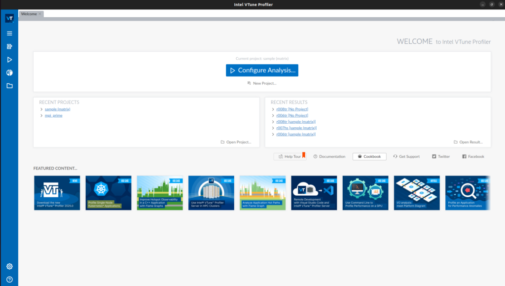
Now we can click on “Configure Analysis” or can create a “New project”. If we click on “Configure Analysis”, we should be able to see following window.
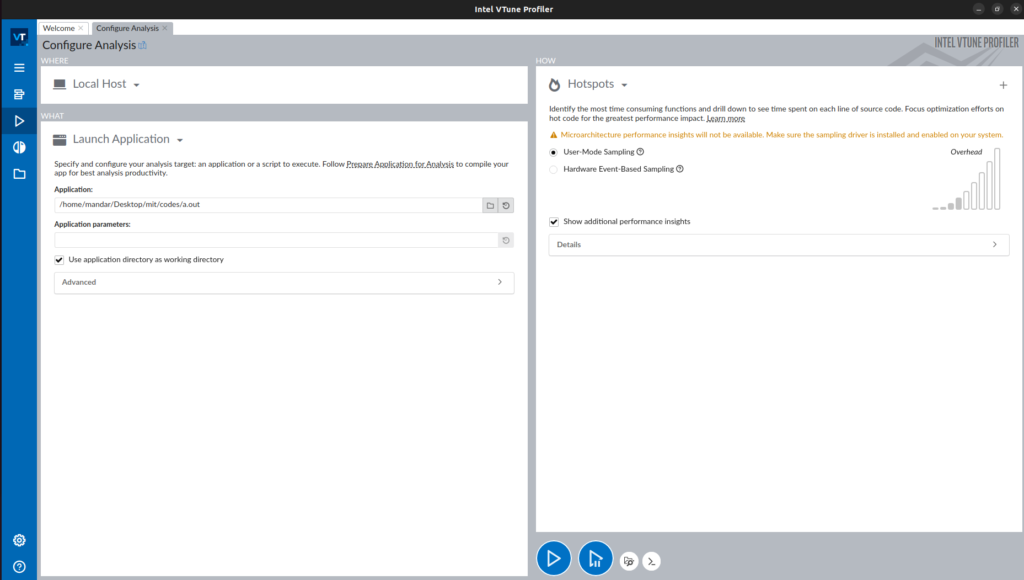
On left hand side, we can choose “Local Host” or other target systems. Just below this, we have option to provide application details.
We can “Launch Application” and profile our code. We need to specify the path to the executable and command line parameters(if any).
On Right hand side we can choose the different analysis types. Screenshot for different analysis types is given below.
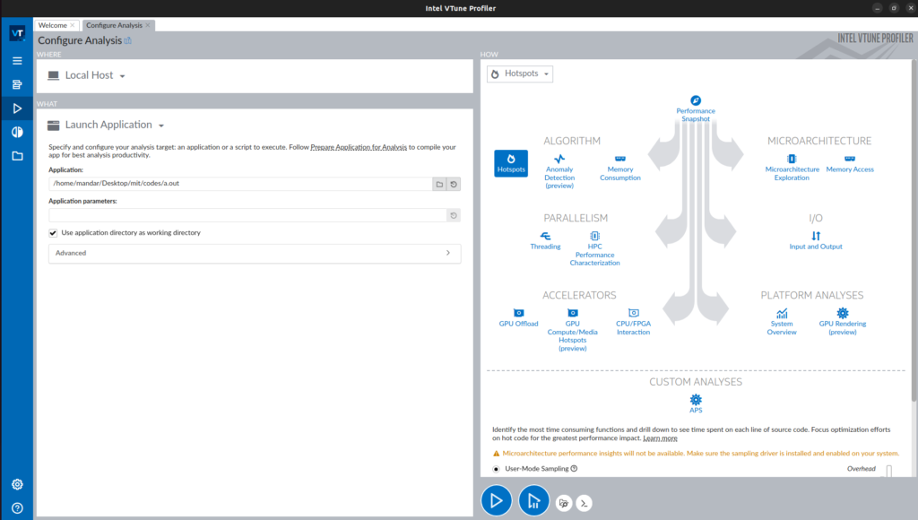
We can specify the application details and choose “Hotspots” analysis. Click on the “Start” button ![]() at the bottom to start the profiling.
at the bottom to start the profiling.
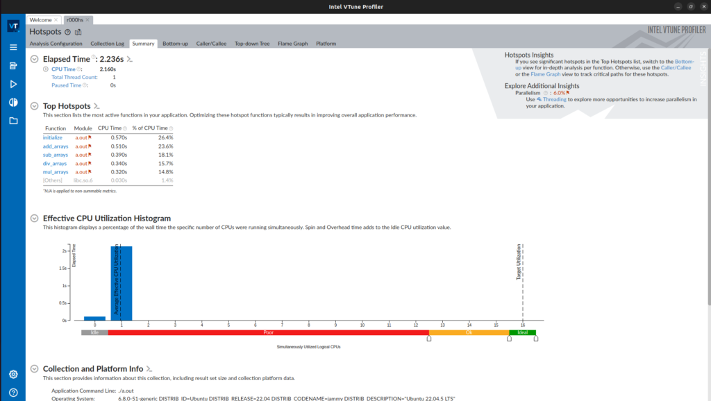
Above window will be shown once the profiling is complete. It shows the summary of the profiling. If we click on the “Bottom-up” tab at the top, we should be able to see following output –
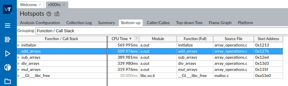
It lists different functions and their execution timings. The functions are listed in descending order.
Based on this list, we can target the most time consuming functions for parallelization and optimization.
If you are interested in more articles on profiling you can find them on this page.